
Random steering is often a useful for simulating interesting steering motion. In this post we look at components that make up a random steering toolkit. These can be combined in various ways to get agents to move in interesting ways.
You might want to have a look at Craig Reynolds’ Steering Behaviour for Autonomous Characters — the wander behaviour is what is essentially covered in this tutorial. The main difference is that we control the angle of movement directly, while Reynolds produce a steering force. This post only look at steering — we assume the forward speed is constant. All references to velocity or acceleration refers to angular velocity and angular acceleration.
Whenever I say “a random number”, I mean a uniformly distributed random floating point value between 0 and 1.
1. Angular displacement, velocity and acceleration
These are the variables we can alter to make the agent steer. For a fuller treatment of these basic quantities, see Basic Rotational Quantities. You might also like to check the Wikipedia article Random Walk.
Angular Displacement
Angular displacement is simply the current angle of the agent (relative to some fixed direction, such as the positive x-axis).
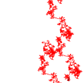
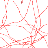
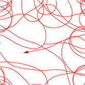
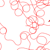
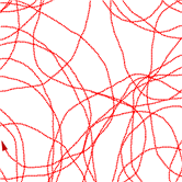
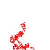
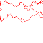
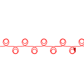
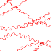
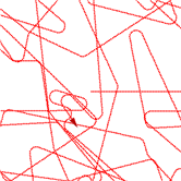
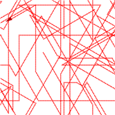
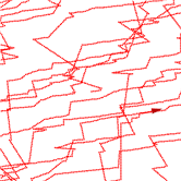
If you decide to make the angular displacement random, you calculate the new angle as:
angular_displacement = 2*max_displacement * (random() – 0.5)
 |
||
| Motion produced by randomly altering the angular displacement. |
As can be seen from the graphic above, the result is very erratic, and not very organic. We can get a better impression of intent if we limit the angles in a certain range (by setting the max_displacement to a lower value than 180), as shown below.
 |
 |
 |
| Same as above, but with angle limited witin 10 degrees of the original displacement. | Angle limited to 30 degrees. | Angle limited to 90 degrees. |
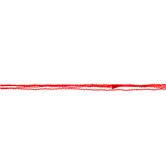
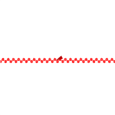
Angular Velocity
Angular velocity is the difference between two displacements (measured in two consecutive simulation steps).
angular_velocity = angular_displacement1 – angular_displacement0
 |
 |
 |
| Velocity is changed randomly, but clamped at 10 degrees. | Velocity clamped at 40 degrees. | Velocity clamped at 80 degrees. |
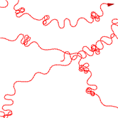
Changing the velocity results in smoother behaviour. The smoothness depends on the maximum allowed velocity.
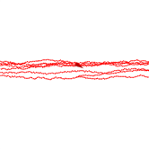
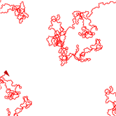
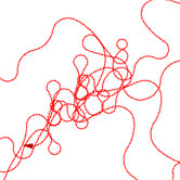
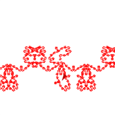
Angular Acceleration
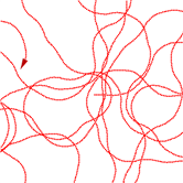
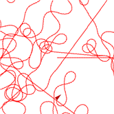
Angular acceleration is the difference between two velocities (measured in two consecutive simulation steps).
angular_acceleration = angular_velocity1 – angular_velocity0
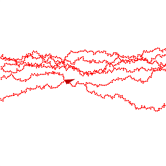
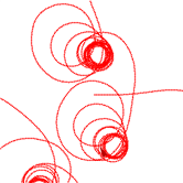
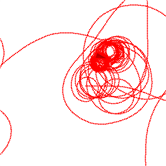
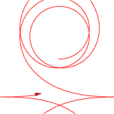
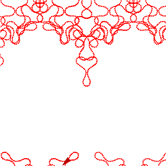
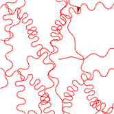
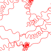
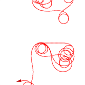
Changing the acceleration is even smoother than changing the velocity. If the acceleration is not clamped to a suitably low value, the agent might go off on a spin for a long time (read the Random Walk article on Wikipedia to understand why).
 |
 |
 |
| Acceleration modified randomly. Acceleration clamped at 0.5 degrees. Velocity clamped at 5 degrees. | Acceleration clamped at 1 degree. Velocity clamped at 5 degrees. | Acceleration clamped at 1 degree. Velocity clamped at 5 degrees. |
 |
 |
 |
| Acceleration clamped at 0.5 degrees. Velocity clamped at 10 degrees. | Acceleration clamped at 1 degree. Velocity clamped at 10 degrees. | Acceleration clamped at 1 degree. Velocity clamped at 10 degrees. |
 |
 |
 |
| Acceleration clamped at 0.5 degrees. Velocity clamped at 15 degrees. | Acceleration clamped at 1 degree. Velocity clamped at 15 degrees. | Acceleration clamped at 1 degree. Velocity clamped at 15 degrees. |
 |
||
| Shows a situtation where the clamped acceleration is not low enough. |
2. Distributions
Changing the distribution of the random numbers we use changes the motion.
Smooth Noise
Smooth noise is generated from uniformly distributed random numbers (white noise) by interpolating values.
For example, the sequence 0 1 0 0 can be smoothed out to 0 0.5 1 0.5 0 0 0, or for smoother result 0 0.25 0.5 0.75 1 0.75 0.5 0.25 0 0 0 0 0.
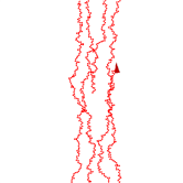
Perlin Noise
Perlin noise is very suitable for rugged organic types of motion. I won’t cover how to produce Perlin noise — see this tutorial.
Arbitrary Distributions
We can also use a handcrafted distribution curve. See the post Generating Random Numbers with an Arbitrary Distribution.
Discrete Distributions
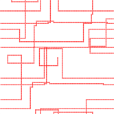
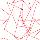
Instead of allowing all angles, we can limit the angles to a discrete set, for example only angles in the set 0, 90, 180, 270. Motion generated from a discrete set is very mechanical.
We can also map Perlin noise to a discrete set, leading to an agent that follows a direction for a longer time.
 |
 |
|
| Smooth noise. | Perlin noise. | |
 |
 |
 |
| Arbitrary distribution curve used to modify displacement. | Arbitrary distribution curve used to modify velocity | Arbitrary distribution curve used to modify acceleration |
 |
 |
 |
| Discrete distribution (90 degrees). | Discrete distribution (60 degrees). | Discrete distribution (30 degrees). |
 |
 |
 |
| Discrete Perlin (90 degrees). | Discrete Perlin (60 degrees). | Discrete Perlin (30 degrees). |
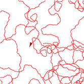
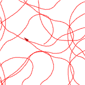
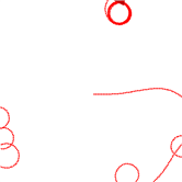
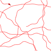
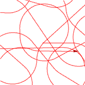
3. Vector Fields
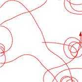
Random vector fields can be useful in certain cases. In general, it is impractical to generate a random vector for each pixel. Instead we generate vectors for a sample grid (say every 10th pixel in every 10th row), and use interpolation for the other pixels. The lower our sampling rate (i.e. the further sample pixels are apart) the smoother the motion will be.
- When setting the angular displacement from such a field, the agent will retrace a path whenever it visits a pixel that has already been visited. This can sometimes be distracting. It is easily fixed by offsetting the angle with a small random amount.
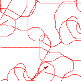
- Random vector field can have sinks from which the agent cannot escape. This is especially true when the acceleration is set from a vector field. One way of resolving this problem is to switch between two or even three vector field at regular intervals. (It can be difficult to reliably detect when the agent is stuck).
 |
 |
 |
| Vector field used to alter displacement. | Vector field used to alter velocity. | Vector field used to alter acceleration. |
 |
||
| Shows a sink in the vector field that permanently traps an agent. |
Vector fields can also be used to bias random numbers. This is useful when the vector field represents landscape features. Thus the field will only “influence” the behavior of an agent, and not control it directly. One very easy way to do this is to use the following formula to adjust the angle:
displacement = r_1 * vec(x, y) + (1 – r_1) * r_2
Where vec(x, y) is the angle obtained from the vector field (possibly interpolated as described above), and r_1 and r_2 are two random numbers.
4. Functions
Instead of using random numbers, we can use functions that depend on time. These functions can be parameterised with random numbers.
The sine function have properties that makes it very convenient to use for this purpose:
- It is smooth.
- Its range (the amplitude) is limited, and easily adjusted with a parameter.
- The frequency is constant and easily tweaked with a parameter, making it easier to control things such as loops when combining different sine functions.
- Different sine functions can be added to lead to complex motion.
- It is easy to blend two sine functions with another function to simulate frequency changes (for example, A(t) * sin(10t) + (1 – A(t)) * sin(t) without unwanted phase effects. Alternatively, the blending can be done with a Perlin noise sequence.
Saw tooth functions and square wave functions have all these properties, except that they are not smooth.
In the images below, the parameter t is incremented each time step.
sin(t) + sin(10t) + sin(50t)
 |
 |
 |
|
| sin(t) | sin(10t) | sin(50t) | |
 |
 |
 |
|
| sin(t) + sin(10t) + sin(50t) | 0.5sin(t) + 0.3sin(10t) + 0.2sin(50t) | 0.5sin(t) + 0.5sin(50t) | |
 |
 |
 |
|
| 0.9perlin_noise(t)sin(t) + 0.1perlin_noise(T – t)sin(50t) | 0.5perlin_noise(t)sin(t) + 0.5perlin_noise(T – t)sin(50t) | ||
 |
 |
 |
|
| white_noise(t) * [0.5sin(t) + 0.5sin(50t)] | smooth_noise(t) * [0.5sin(t) + 0.5sin(50t)] | perlin_noise(t) * [0.5sin(t) + 0.5sin(50t)] |
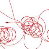
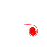
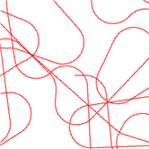
5. Timed Transitions
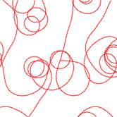
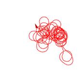
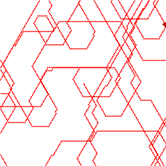
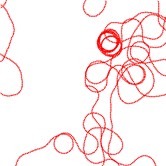
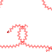
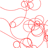
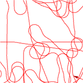
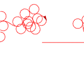
Instead of changing the angular displacement (or velocity or acceleration) at every time step, we can change it only every “once in a while”. For example, we can change it when a fixed number of time steps have passed. More interestingly, we can change it only when a random number of time steps have passed.
The presence of many circular loops indicate long times of constant velocity. When we adjust the velocity or acceleration, this can happen when the intervals are too long in relation to the max angular velocity. When we adjust the acceleration, it can also happen when the max velocity is too low relative to the maximum acceleration – leading to quick “saturation”.
When combined with angles from a discrete distribution, we get the machine-like behaviour (similar to using Perlin noise mapped to a discrete set as above).
 |
 |
 |
| Displacement | Velocity | Acceleration |
 |
 |
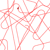 |
| Clamped velocity (low). | Clamped velocity (medium). | Clamped velocity (high). |
 |
 |
 |
| Clamped velocity (very high). | Clamped acceleration and velocity (low velocity). | Clamped acceleration and velocity (high velocity). |
 |
 |
 |
| Discrete set (90 degrees). | Discrete set (72 degrees). | Very regular movement when clamped acceleration is low relative to the clamped velocity. |
6. Transition Tables and Functions
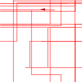
Sometimes we would like to change the distribution of a randomly generated angle based on the current steering angle. We can use transition tables for this.
| <15 | 15< <30 | 30< | |
| <15 | 0.9 | 0.07 | 0.03 |
| 15< <30 | 0.15 | 0.8 | 0.05 |
| 30< | 0.1 | 0.2 | 0.7 |
The table above is an example of a transition table. It basically describes the probability that if the current steering angle is within a certain range, it will change to some other range. For example, if the current steering angle is smaller than 15 degrees, there is a probability of 0.9 that the next angle will also be smaller than 15 degrees. If the angle is greater than 30 degrees, the next angle will be smaller than 15 degrees with a probability of 0.1.
To implement this, we convert the probability table above to a accumulative probability table, where we sum over rows, like this:
| <15 | 15< <30 | 30< | |
| <15 | 0.9 | 0.97 = 0.9 + 0.07 | 1 = 0.9 + 0.07 + 0.03 |
| 15< <30 | 0.15 | 0.95 = 0.15 + 0.8 | 1 = 0.15 + 0.8 + 0.15 |
| 30< | 0.1 | 0.3 = 0.1 + 0.2 | 1 = 0.1 + 0.2 + 0.7 |
Now, at each simulation step, we check the current angle, and choose the appropriate row of the table to work with. Now we generate a (uniformly distributed) random number. Then we check it against the values in the row. The left most cell that is bigger than the random number is the one we want to work with – it denotes the range of the new angle. Then we simply generate a random number in this range. In practice we don;t need the last column.
The table above can be interpreted as follows:
- if the current angle is in a certain range, the probability is high that it will be again in that range;
- if the range changes, it will more likely change to an adjacent range; and
- if the range changes and there are two adjacent ranges, the left one is favored.
We can smooth out the results by using a 2D response curve, but this can be tricky. Also, we need to specify many values to get the 2D distribution we want.
In a special case we can follow a two step process instead. We use two tables:
- one to describe the probability that an angle will change (base on the angle size);
- and a simple transition table as above.
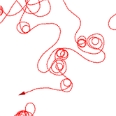
This leads to fairly regular movement, as shown in the figures.
 |
 |
 |
| Agent using the transition table above. | Agent using the transition table above but only change angles with probabilities 0.1, 0.2, 0.4 for the tree angle ranges. | Agent using the transition table above but only change angles with probabilities 1, 1 0.1 for the tree angle ranges. |
7. Paths
It is sometimes easier to steer towards a generated path than to control the steering directly. Using paths have several advantages:
- the agent’s future movement is always known, making it easier to predict; and
- paths can be saved, and transmitted over a network. This can make it easier to keep networked simulations (such as multiplayer games) in synch, and support features that require determinism (such as replay).
Steering on a path is covered in Reynold’s paper – here we look at a two simple random path generating algorithms.
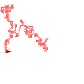
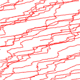
Fractals
A simple path generating algorithm generates fractals:
- Start with a single segment – two points in a list
- For each pair of adjacent points in the list (each representing a line segment), add some intermediate points (based on some algorithm – see below)
- Repeat until the result is suitably detailed.
The algorithm used to generate new points will determine the characteristics of the final path. Here are a few examples:
- For each point pair, generate a random point close to the midpoint.
- For each point pair, generate two points close to the third and two third points, on opposite sides.
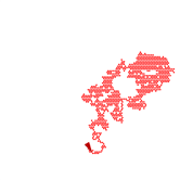
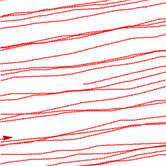
Functions
Start with a line, a circle, or some other simple figure, and add sine functions to it. For example, a circle’s equation in polar coordinates is:
r = k
We can now add sine waves, like this:
r = k + r_1*sin(t) + r_2*sin(2t) + r_3*sin(4t) + …
r_i can be chosen constants, or randomly generated numbers.
Again, saw tooth and square wave functions are also suitable for adding to the base path. Other functions can also be used, although you should take care that they stay witin a predefined range.
Download
Random Motion Game Maker File
Most of the principles discussed here have been implemented in the following Game Maker file:
random_movement.gmk 180 KB
Read the README file in the scripts folder (inside the Game Maker file).
Reynolds’ Open Steer Library
This is a C++ implementation of Reynolds’ steering behaviours that can be plugged into a game or simulation.
Links
- Flipping you the Boid (ActionScript swarming behaviour demo – with source code).
- Agents, Behaviour, Emergence and Embodiment (a list of resources).
- Simulating Crowd Dynamics: Flow Lanes and Character Animation.
- Simulation and Visualization of Agents in 3D Environments (PDF 1.61 MB).
- Steering a Virtual Crowd Based on a Semantically Augmented Navigation Graph (PDF 3.96 MB).
- A Microscopic Swarm Model Simulation and Fractal Approach towards Swarm Agent Behaviour (PDF 622 KB).
- The Experiments for Exploring Dynamic Behaviors in Urban Places (PDF 12.83 MB).
- Simulating Crown Behaviour in Computer Games (PDF 621 KB).
- Towards Building an Intelligent Traffic Simulation Platform (PDF 154 KB).
- Tank Wars (PDF 435 KB).
- REACT: Crowd Simulation System for Visual Effects (PDF 846 KB).
- Hybrid Representations and Perceptual Metrics for Scalable Human Simulation (PDF 5.39 MB).
Great post!
It’s amazing how this steering stuff is always on the borderline between art and science. Just goes to show how long it can take to tweak the motion so that it looks just right in a game!
Oh, and thanks for the link too.
Alex
AiGameDev.com
Thanks 😉
I think it is exactly this borderline art-science effect that makes motion so compelling – and why adding a bit of motion (animals or machines) can do so much for a scene. But like you said – tweaking it can be very difficult, especially if you do not understand the range and limitations of the system you are trying to tweak.
ht
For things like AAA games with character animations, all this steering stuff goes out of the window for this reason; it’s far easier to tweak animations and motion-capture data, along with a motion synthesis algorithm, than it is to rely on steering to provide natural patterns. (Though I’d definitely use steering for non-human characters.)
Alex
AiGameDev.com
Brilliant read!!!
U know what you do so well! U keep a mere artist like me, interested in the programming side of everything!!!
Great post!!!
@Alex: Tweaking can be the death of any complex system. On the racing games I worked on, I had to replace “sophisticated” analytical systems with just telling the vehicle what to do by tagging the road with instructions everywhere – because I couldn’t tweak the “sophisticated” system to work… So I can totally understand how steering algorithms can fall short for human motion.
@Byder: In the end programming under the hood is just a private (almost secret) satisfaction; it is all about how that is perceived (visually, mostly) that counts… glad I help to keep that interest! 😉
Very True! With out you guys, we artists may as well be drawing on paper!!
C 😀
Game Dev Journal