May 5, 2024 A simple color map algorithm I have had to manipulate a lot of images in my life to look nice with brands where no designer was available to do…
August 14, 2022 Implementing and using buffers in C# You can find implementations of the data structures described here at: A buffer is a simple data structure that allows you to add any…
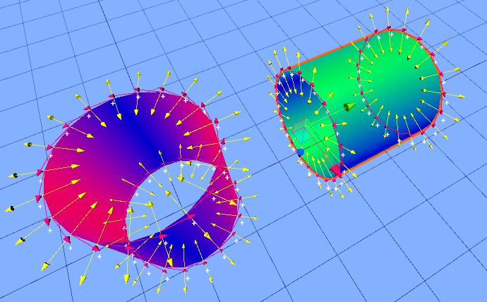
November 25, 2020 Procedural Meshes in Unity: Normals and Tangents In previous posts, we looked at general mesh generation in Unity, and the issues that arise in generating meshes for lines. In this post,…
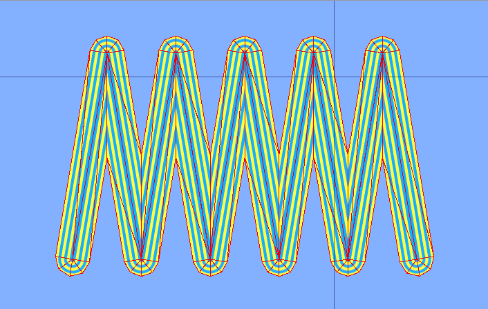
November 10, 2020 Procedural Meshes for Lines in Unity A lines is a fundamental graphics object, but generating attractive, robust lines involve many subtle issues and can be difficult to get right. In…
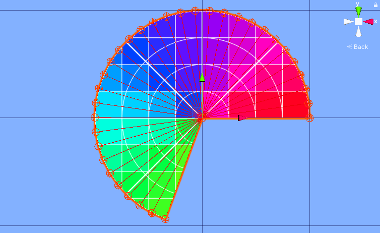
November 4, 2020 Generating meshes procedurally in Unity Procedurally generated meshes have several uses in game development: You can use them for crisp, non-standard UI components. You can use them to render…
July 22, 2018 Domino Tilings I I started a new project: studying polyomino tilings and related problems (very much inspired by Golomb’s famous Polyominoes). As part of this study, I…
February 18, 2016 Generators A generator (as I will use the term here) is an object that can “generate” other objects on demand. They work like random generators,…
January 24, 2011 2D Minimum and Maximum Filters: Algorithms and Implementation Issues A while back I needed to implement fast minimum and maximum filters for images. I devised (what I thought was) a clever approximation scheme where…
July 27, 2010 A Simple Trick for Moving Objects in a Physics Simulation (Original Image by Valerie Everett) It is sometime necessary to move an object in a physics simulation to a specific point. On the one…
June 15, 2010 Region Quadtrees in C++ (Original image by GoAwayStupidAI). Below are four C++ implementations of the region quadtree (the kind used for image compression, for example). The different implementations…